Oracle Manipulation 101 (Math edition)

12/26/22

Author: Parti

Intro

This article is divided into two.

In the first part, we will present a quick refresher on how Uniswap works specifically tailored to the needs of computing manipulation costs. It'll explore how to move the spot price in an AMM to the desired target for Uniswap v2 and v3.

The second part will show how we obtained the results from the "Oracle Manipulation 101" article. To do so, we will present step-by-step an attack of a lending protocol in DeFi. This case can be later generalized to different types of markets.

You can follow along with the simulations provided in this colab.

Uniswap Math

There are many great resources on the topic of Uniswap. We will show some definitions and then present new results for price manipulation in Uniswap v3.

Full Range and Uniswap v2

Let's begin by looking at Uniswap v2 AMMs, equivalent to a Full Range position in Uniswap v3. Note that we'll confirm this below.

Basic equations

Two different tokens' balance forms each "pool". Users can add balance to these pools and later remove it. Let's call $x$ the balance of token A and $y$ the balance of token B. The following equation gives the relationship among these balances:

$x*y=L^2 \hspace{1cm}(1)$

where $L$ is called Liquidity. This $L$ is modified only when someone adds or removes the token balance and is constant otherwise.

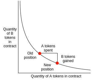
Anyone can swap token A for token B or vice versa on this pool, modifying the balances $x$ and $y$ in the pool according to $(1)$. You can visualize this behaviour in the Figure (source).

We can compute the price of token A relative to token B at which anyone buys tokens from any AMM (not only constant product type) as

$P_{A/B}=-\frac{dy}{dx} \hspace{1cm}(2)$

The way to think about this formula is to picture a user selling a quantity $dx$ of token A to the pool. The pool reserve will increase $dx$ for token A while decreasing $-dy$ for token B. The ratio will yield the price at which the user sold their token A amount. This paper explains how Eq. $(2)$ and an invariant are all we need to build an AMM.

From $(1)$ we have $y=\frac{L^2}{x}$. Then

$P_{A/B}=-\frac{d}{dx}(\frac{L^2}{x})=\frac{L^2}{x^2} =\frac{y}{x} \hspace{1cm} (3)$

The price for Uniswap v2 pools can be computed as the ratio among the balances of the two tokens. So, for instance, if the WETH/USDC pool has $2$ WETH and $4000$ USDC, the price of WETH can be computed as $P_{WETH/USDC} = \frac{4000}{2}=2000$. This expression is, of course, symmetrical to the exchange of labelling, so to compute the price of USDC relative to WETH in the previous example, we invert the equation $(3)$:

$P_{USDC/WETH} = \frac{2}{4000}=0.0005=\frac{1}{P_{WETH/USDC}}$

Notice we can also describe the pool using liquidity and price instead of token balances. Using $(3)$:

$P = \frac{y}{x} = \frac{L^2}{x^2}\rightarrow x = \frac{L}{\sqrt{P}}$

$P=\frac{y}{x}=\frac{y^2}{L^2}\rightarrow y = L\sqrt{P}\hspace{1cm}$

Price manipulation

Let's make a swap and see how the price moves. Suppose Alice wants to buy token B from the AMM with liquidity $L$ with $\Delta x$ token A. Then:

$(x+\Delta x)(y-\Delta y)=L^2=xy$

Alice gets an amount $\Delta y$ of token B in return:

$\Delta y = y(\frac{\Delta x}{x+\Delta x})$

The final price of token A relative to token B is:

$P_f = \frac{y-\Delta y}{x+\Delta x}= \frac{L^2}{(x+\Delta x)^2}$

From where can we recover

$\Delta x = \frac{L}{\sqrt{P_f}}-x = L(\frac{1}{\sqrt{P_f}}-\frac{1}{\sqrt{P_i}}) \hspace{1cm} (4)$

where $P_i$ is the initial price of token A relative to token B. Eq. $(4)$ tells us exactly how much $\Delta x$ Alice needs to move the spot price from $P_i$ to $P_f$ given the liquidity.

Similarly, if Alice wanted to buy token A with $\Delta y$ token B:

$(x-\Delta x)(y+\Delta y)=L^2=xy \rightarrow \Delta x = x(\frac{\Delta y}{y+\Delta y})$

$P_f = \frac{y+\Delta y}{x-\Delta x}=\frac{(y+\Delta y)^2}{L^2}$

And we get to

$\Delta y = L\sqrt{P_f}-y = L(\sqrt{P_f}-\sqrt{P_i})\hspace{1cm} (5)$

You can play around with these formulas in this link.

Uniswap v3

Uniswap v3 revolutionized how AMMs work. The whitepaper goes in-depth on it, but the key takeaway is that liquidity can now be deployed over particular price ranges, unlocking a new level of capital efficiency.

Basic equations

Eq. $(1)$ gets replaced by the following formula

$(x+x_{offset})(y+y_{offset})=L^2,\quad\quad x_{offset}=\frac{L}{\sqrt{p_{upper}}},\quad y_{offset}=L\sqrt{p_{lower}}\hspace{1cm}(6)$

The equation is misleading, as liquidity can change for different price ranges. Eq. $(6)$ is valid for each range where liquidity is constant and adjusts accordingly each time the price moves to a different liquidity region. We will dig deeper into it below.

Notice first that a Full Range liquidity position corresponds to taking the limits $p_{lower}\rightarrow 0$ and $p_{upper}\rightarrow \infty$. Doing so would eliminate the offsets and make $(6)$ equal to $(1)$. That's why a Full Range position in Uniswap v3 is equivalent to a Uniswap v2 position. Uniswap v3 does not reach prices of zero and infinity, but it's an excellent approximation.

We can solve $(6)$ for $x$ and $y$:

$x=\frac{L^2}{y+y_{offset}}-x_{offset},\quad y=\frac{L^2}{x+x_{offset}}-y_{offset} \hspace{1cm}(7)$

We can compute the price as

$P=-\frac{dy}{dx}=\frac{L^2}{(x+x_{offset})^2}\rightarrow \sqrt{P}=\frac{L}{x+x_{offset}}=\frac{y+y_{offset}}{L} \hspace{1cm}(8)$

As a corollary, we can also obtain the following interesting result.

$y=L\sqrt{P}-y_{offset}\rightarrow L=\frac{dy}{d\sqrt{P}}$

Heuristic approach

When dealing with Uniswap v3, it's easy to get lost in equations and forget the big picture. It's essential to have a clear image of what's going on to develop the "Unintuition".

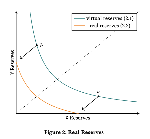
One way of understanding Uniswap v3 is as a union of different Uniswap v2 pools for different price ranges. Analogously, we can think of it as a single Uniswap v2 pool but where liquidity is a split function such that:

$L(price)=\begin{cases}L_0,\quad price<p_0\\ L_1,\quad p_0<price<p_1\\ \vdots\\ L_N,\quad p_N<price \end{cases}$

the terms $x_{offset}$ and $y_{offset}$ are only centring the equation in the corresponding range, as you can see in the Figure from the whitepaper:

Understanding Liquidity

The LP is composed of a single asset when providing liquidity outside the current price range. Once deployed, the position will remain idle until the pool price reaches the edges. Only when the price falls inside will the balance of each asset follow Eq. $(6)$. Single-sided positions are often considered sell or buy orders, as swapers will convert them to the other asset once the price moves over. This interpretation is not strictly right, as the bought asset would convert back if the LP did not remove the position and price returns. We can find a better analogy in options.

Liquidity is not straightforward to compute now, as its formula depends on the price range. If we call the current price $P$ and the edge prices of the position $p_{lower}$ and $p_{upper}$, then

1. When $P\leq p_{lower}$, position is fully token A ($y=0$): $(x+\frac{L}{\sqrt{p_{upper}}})L\sqrt{p_{lower}}=L^2$ $x=L(\frac{1}{\sqrt{p_{lower}}}-\frac{1}{\sqrt{p_{upper}}})=L\frac{\sqrt{p_{upper}}-\sqrt{p_{lower}}}{\sqrt{p_{lower}}\sqrt{p_{upper}}}$ $L_x\equiv L=x\frac{\sqrt{p_{lower}.p_{upper}}}{\sqrt{p_{upper}}-\sqrt{p_{lower}}}$
2. When $P\geq p_{upper}$, all position is made of B ($x=0$): $\frac{L}{\sqrt{p_{upper}}}(y+L\sqrt{p_{lower}})=L^2$ $y=L(\sqrt{p_{upper}}-\sqrt{p_{lower}})$ $L_y\equiv L=\frac{y}{\sqrt{p_{upper}}-\sqrt{p_{lower}}}$
3. When $p_{lower}<P<p_{upper}$, Uniswap calculates the minimum between $L_x$ and $L_y$: $L=min[L_x,L_y],\quad L_x=x\frac{\sqrt{P.p_{upper}}}{\sqrt{p_{upper}}-\sqrt{P}},\quad L_y=\frac{y}{\sqrt{P}-\sqrt{p_{lower}}}$ Here, $L_x$ is the liquidity provided by asset $x$ in the range $(P,p_{upper})$ and $L_y$ is the liquidity provided by $y$ in the range $(p_{lower},P)$. An optimal position in such a scenario corresponds to $L_x=L_y$: $L_x=L_y\rightarrow x\frac{\sqrt{P.p_{upper}}}{\sqrt{p_{upper}}-\sqrt{P}}=\frac{y}{\sqrt{P}-\sqrt{p_{lower}}}$ which can be solved for $x, y, P, p_{lower}$ or $p_{upper}$ without speaking of liquidity.

You can find the full code implementation in this link. You can play around with different values here. Also, you can find examples here and here.

Price Manipulation

We can do the same math we did for Full Range positions to figure out how much capital is required to manipulate a pool to a target spot price (Eqs. $(4)$ and $(5)$). To do so, we have to divide the range over the edges where the underlying liquidity changes. We can arrange these edges in a vector $p_{edge}=[0,p_1,\dots,p_N,\infty)$ ($0$ and $\infty$ are not exact but concept-approximations, as there are a minimum and a maximum allowed price in Uniswap v3). Let's assume we are on a price $P$ between edges $p_i$ and $p_{i+1}$.

1. If moving the price of token A relative to token B to the upside: We have to dump token B. Here $y_i$ are the initial reserves of token B in the active range. - We can first compute how much capital we need to move the price to the following edge $p_{i}$. Using $(8)$: $\frac{p_{i+1}}{P}=\frac{(y_i+\Delta y_1+y_{offset\,i})^2}{(y_i+y_{offset\,i})^2}$ $\sqrt{\frac{p_{i+1}}{P}}=\frac{(y_i+\Delta y_1+y_{offset\,i})}{(y_i+y_{offset\,i})}$ $\Delta y_1 =(y_i+y_{offset\,i})(\sqrt{\frac{p_{i+1}}{P}}-1)$ - From here, we compute how much capital is required to reach the following edge $p_{i+2}$: $\Delta y_2=(y_{i+1}+y_{offset\,i+1})(\sqrt{\frac{p_{i+2}}{p_{i+1}}}-1)$ But $y_{i+1}$ is the balance of token B when the position crosses the liquidity range, which equals zero. Hence $\Delta y_2=y_{offset\,i+1}(\sqrt{\frac{p_{i+2}}{p_{i+1}}}-1)$ We can use this same procedure for the following edges - Finally, to reach the target price $P_f$ from the last crossed edge $p_j$: $\Delta y_j=y_{offset\,i+j-1}(\sqrt{\frac{P_f}{p_{i+j-1}}}-1)$ Then we have: $\Delta y=\sum_{l=1}^j\Delta y_l,\quad \Delta y_l = \begin{cases}(y_i+y_{offset\,i})(\sqrt{\frac{p_{i+1}}{P_i}}-1) & l=1\\ y_{offset\, i+l-1}(\sqrt{\frac{p_{i+l}}{p_{i+l-1}}}-1)&l\neq 1,l\neq j\\ y_{offset\, i+j-1}(\sqrt{\frac{P_f}{p_{i+j-1}}}-1)&l=j \end{cases}\hspace{1cm} (9)$

   where $j$ is a function of the final price and the liquidity edges¹.
   

2. If moving the price of token B relative to token A to the downside: We have to dump token A. The reasoning is the same but in the other direction.

$\Delta x=\sum_{l=1}^j\Delta x_l,\quad \Delta x_l = \begin{cases}(x_i+x_{offset\,i})(1-\sqrt{\frac{p_{i}}{P}}) & l=1\\ x_{offset\, i-l+1}(1-\sqrt{\frac{p_{i-l+1}}{p_{i-l+2}}})&l\neq 1,l\neq j\\ x_{offset\, i-j+1}(1-\sqrt{\frac{P_f}{p_{i-j+2}}})&l=j \end{cases}\hspace{1cm} (10)$

It is possible to compute the cost of manipulation analytically. Still, to do so, it's necessary to keep track of every liquidity and its edges, which can be done via direct pool querying or using indexers like The Graph. An alternative to this is to use a brute-force search (Euler has built an excellent implementation of this approach).

1: Guillaume Lambert made me notice that for arbitrary Uni v3 positions, this can be taken to a closed form:$\Delta y = \int_{P_i}^{P_f}((r-1)/√r * √P * L(P)) dP$, where $r=\sqrt{\frac{P_b}{P_a}}$ with $P_a$ and $P_b$ the edges of each position. This expression assumes each position was deployed centered around $K=\sqrt{P_aP_b}$

Concentrated liquidity and price manipulation

With high power comes high responsibility: compared to Full Range liquidity, concentrated liquidity is excellent at increasing the potential LP return, but it also means manipulating the price gets easier. The most straightforward way to think about it is that the concentrated LP sells its capital at a lower average price than a Full Range. This affirmation is not always true, but it is for sure when the position is in the active region.

It is possible to make manipulation more expensive through concentrated positions by placing them far away from the current price. Still, there are no incentives to do so (this position would receive zero fees).

On top of that, concentrated liquidity is more prone than Full-Range to move from pool to pool to seek a higher APY.

For all these reasons, when evaluating the safety of Uniswap-based oracles, Full Range positions are strongly encouraged and taken into account over concentrated positions (see here and here).

The problem is, not even Full Range positions can be considered secure with current models. Remember that oracle users often differ from protocols that provide liquidity for their token. A lending market that accepts a specific token as collateral cannot know if the available full-range position will stay and cannot assign higher tiers/LTVs to them. This issue is one of the main points that PRICE solves.

In the analysis, we will only consider the Full Range positions, as

1. It's consistent with the above liquidity visibility and security claims.
2. We will require committed Full-Range positions for the oracle to work. When adding concentrated positions on top, the manipulation cost will only increase so that the analysis will serve as a worst-case scenario.

But what about positions which are almost Full Range? Well, that's an exciting topic. When manipulating a price, no one takes the price to infinity or zero, and deploying only over this range will surely increase capital efficiency. This claim is valid but requires knowing at which price a manipulation stops being profitable, which is not universal: it's a function of each market's parameters and the attacker's available capital.

PRICE will likely incorporate semi Full Range positions in future versions, but always with a mandatory Full Range position below.

TWAPs

Uniswap knows its role as a decentralized on-chain price source and has built its contracts to accommodate this fact. With the current version, price queries return a mathematical object known as $TWAP$. An attacker must consider this when manipulating a price. But what is a $TWAP$? Let's dive in.

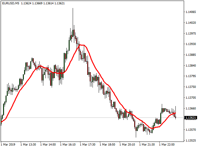
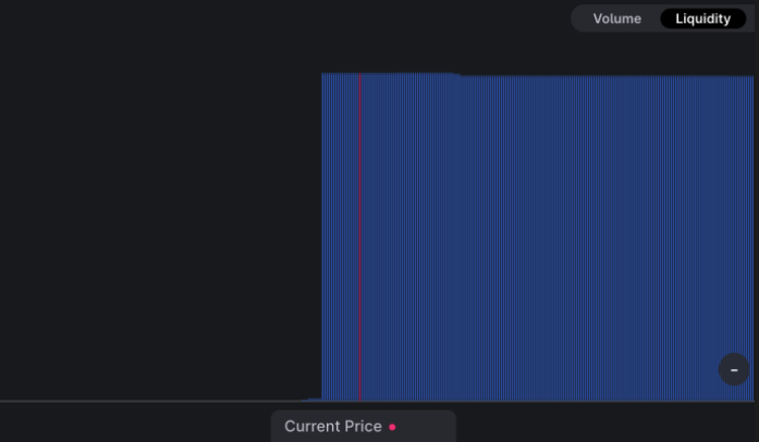
$TWAP$ stands for time-weighted average price. It's a geometric average price for a pool over a fixed interval of time and is what we query from the current implementation of the Uniswap v3 Oracle library. It's also a standard trading tool, as seen in the red line in the Figure.

ℹ️ Given 2 numbers, $a_1$ and $a_2$: Arithmetic mean: $\frac{a_1+a_2}{2}$ Geometric mean: $\sqrt{a_1*a_2}$

This can be easily generalized over $N$ numbers $a_i$ as Geometric mean: $\sqrt[N]{\prod_{i=1}^N a_i}$

Each pool on Uni v3 keeps track of an array which stores historical information about the price (the "ticks" formally) and the time duration of it, together in the "accumulator" values (summation of the ticks times each elapsed time). The array has a fixed length (cardinality) and overwrites by "moving" to the right as new observations occur. The longer the cardinality, the more observations can be stored. Pools are initialized with a maximum of one stored observation but can be increased by paying gas to execute a function in the pool's contract.

The observation's array is updated on the block's first swap/liquidity provision (only if in the active range). Observations correspond to the values from the "accumulator" at the end of the previous block. Flash-loan manipulations are hence not recorded. To impact the $TWAP$, attackers would have to expose themselves to arbitrage for a long time, increasing the attack cost. Additionally, swappers and LPs are responsible for paying the gas cost of a price update, sustainably subsidizing the oracle. Truly a giga-brain design by the Uniswap team.

Many resources are available on how the Geometric mean works in Uniswap v3. The key equation to keep in mind is (5.2) from the whitepaper describing the value of the geometric mean time-weighted average price among times $t_1$ and $t_2$:

$P_{t_1,t_2} =\left(\prod_{i=t_1}^{t_2}P_i\right)^{\frac{1}{t_2-t_1}} \hspace{1cm}(11)$

As stored observations are constant in intervales, we can model this equation:

$P_{t_1,t_2}\equiv TWAP_{t_1,t_2} = (\prod_{i=1}^N P_i)^{\frac{1}{N}}$

For some discretization, where $i$ is the index of each discrete interval, $P_i$ the price at each discrete interval, and $N$ is the number of discrete intervals $t_1$ and $t_2$ (for instance, if observations have a duration of $4s, 2s$ and $3s$, $N$ equal to $9$ will be enough to make this formula exact).

It is possible to make an approximation where these constant intervals are Ethereum blocks: this is not exact because it assumes $t_1$ and $t_2$ fall exactly on the observations, which is most commonly not the case, but the error is bounded by the block duration ($12.5s$) on each end. The longer the interval, the more likely it is to have a better approximation, as each observation has less weight. If the price remains constant at $P_1$ for $N-M$ blocks and moves to $P_2$ for $M$ blocks, then

$TWAP_{t_1,t_2} \simeq (P_1^{(N-M)}P_2^M)^\frac{1}{N} \hspace{1cm}(12)$

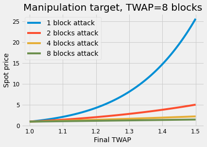
From here, we can deduce a simple formula for $P_2$ as a spot price to achieve a desired $TWAP$ value:

$P_2 \simeq \sqrt[M]{\frac{TWAP_{t_1,t_2}^N}{P_1^{(N-M)}}} \hspace{1cm} (13)$

You can gain more by playing around at this link. Notice the target price behaves similarly to an exponential function with $N/M$ as the exponent (this is not exact due to the divisor). So, as a takeaway:

• Using longer TWAPs will make movements exponentially harder.
• Moving the price over several blocks reduces the costs exponentially.

ℹ️ To manipulate a $TWAP$ to the desired price, an attacker needs to move the spot much more so that the average falls on target. The longer the $TWAP$ length $N$ is relative to the attack's $M$, the harder it is to manipulate. That is why longer $TWAPs$ are suggested for a safer query.

Conversely, taking longer TWAPs means having a laggier query and a less accurate price. This tradeoff between security and precision is one of the main critiques of using Uniswap as an oracle. At PRICE, we have reduced this tradeoff to the bare minimum, eliminating another user headache.

Oracle Manipulation 101 Math

In the Oracle Manipulation 101 article, we have presented a study case for an oracle manipulation analysis. In particular, we have explained how an attack on a lending market can become profitable. This section will show how many of the results we have presented were derived.

As a brief rundown, attacks will likely happen if the profit from manipulation exceeds the cost of manipulation. Understanding this is fundamental to setting the parameters that allow for capital efficiency without adding new risks.

The Cost of Manipulation refers to the capital used ti borrow + capital used to move an AMM's price to the desired target. The latter is what we deduced in the Uniswap Math section above, both for Uniswap v2 and v3. As mentioned in Oracle Manipulation 101, we will consider Full Range positions for this analysis, which is consistent with our previous claims about concentrated positions.

We will exclude trading fees for simplicity of reading, but you can trivially add them to the analysis.

Math for Attack Scheme pre PoS

The regular scheme for attacking a lending market is the following:

1. The attacker will use a total capital $C$ (measured in B): $C=C_{colateral}+C_{manipulation}$
2. With $C_{colateral}$, purchase $a_{colateral}$ of A at price $P_i$ (relative to B): $C_{colateral}=a_{colateral}P_i$. The attacker can do this over several blocks and liquidity markets to mitigate price impact. This step is not necessary if efficient arbitrage exists.
3. With $C_{manipulation}$, manipulate the $TWAP$ to $TWAP_{final}$, by purchasing $a_{manipulation}$ of token A in the AMM. The spot price to manipulate depends on the length of the $TWAP$ queried by the market.
4. Deposit $a_{colateral}$ as collateral and borrow asset B with borrowing capacity $f*a_{colateral}*TWAP_{final}$. Notice the reserves cap this amount. If efficient arbitrage exists, then deposit $a_{manipulation}$ instead.
5. If possible (no arbitrage), manipulate the price back to the starting value by selling back $a_{manipulation}$ (or what's left) of A and get at most $C_{manipulation}$ back. This step makes a huge difference in cost.
6. Default bad debt and profit. Notice the stolen capital B can be sold slowly over time to reduce price impact.

Then, the profit is

$Profit=min[a_{colateral}fTWAP_{final},Reserves+SoldBack]-a_cP_i-C_{manipulation}^*$

Where $C_{manipulation}^*$, the final cost of manipulation depends on point 5, and $SoldBack$ is the exceeding capital sold back to the pool (only greater than zero if reserves were exhausted). Any attack with $Profit>0$ is profitable (equivalent to $f\times TWAP_{final}>1$ if no arbitrage). If arbitrage will happen (step 5 is impossible), then the most efficient strategy is to use the capital obtained from manipulation as collateral.

Before PoS, for relevant enough markets, manipulating the price back to the initial value was extremely unlikely for the attacker for healthy liquidities, as Uniswap v3 Oracle requires a one-block delay to update, exposing the arbitrage opportunity (an explanation on this on the Uniswap refresher). This paper showed that, if efficient arbitrage exists, a single-block attack becomes cheaper to execute than a multi-block attack (results are for Uniswap v2 $TWAP$, but are also valid for v3) for large enough manipulations.

Healthy liquidity

Suppose the attacker knows arbitrage will happen and the pool has a Full Range position with liquidity $L$. In that case, the best plan is to borrow as much as possible (sell high) using the capital obtained from manipulation. What's missing should be swapped for a price close to $P_i$. The cost of this manipulation is

$C_{manipulation}^*=L(\sqrt{P_f}-\sqrt{P_i})$

and the pool returns a token B amount

$\Delta y =y(\frac{\Delta x}{x+\Delta x})$

The attacker will use a part from this $\Delta y$ to borrow (until emptying the reserves) and a part to sell back to the pool. Hence,

$\Delta y = \Delta y_{sell}+\Delta y_{borrow}$ $\Delta y_{borrow}=\frac{Stolen}{fP_f}$

The number of reserves caps the $\Delta y_{borrow}$:

$\Delta y_{borrow}^{max}=\frac{Reserves}{fP_f}$

What's missing will be swapped back $\Delta x_{sell} \simeq P_i\Delta y_{sell}$.

$Profit = \Delta x_{out} - \Delta x_{in} = min[fP_fy(\frac{L\sqrt{P_f}-x}{L\sqrt{P_f}}), Reserves+ \Delta y_{sell}P_i]-C_{manipulation}^*$

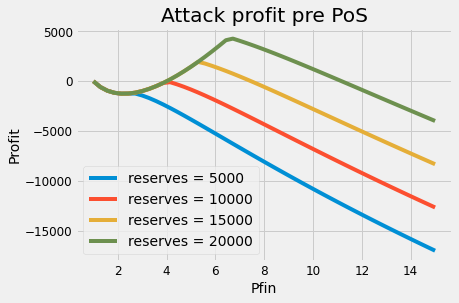
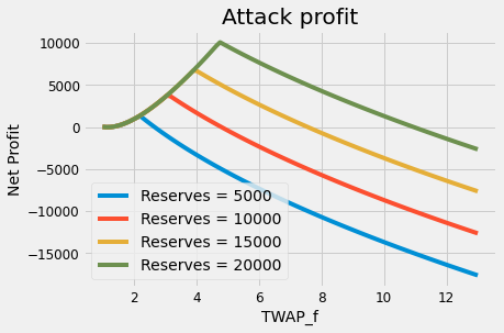
You can play around simulating the arbitrage scenario in this link. You can see in the Figure below that the optimal attack in this scenario will correspond to using all capital from the manipulation to borrow up to the available reserves (no $\Delta y_{sell}$ left). It's possible to find this optimal price analytically as a function of the reserves, which LPs can use to define safe semi Full-Range positions. Notice this graph does not take TWAP into account and is only valid for markets which query the spot price.

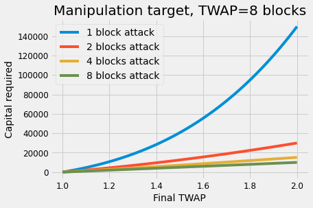
To include the $TWAP$ parameters in the analysis, we should compute the Cost of Manipulation $C_{manipulation}^*$ with the spot price added using Eq. $(3)$ while keeping the $TWAP$ price to obtain the stolen amount. We can also simulate this and check that manipulation cost increase radically to the point where single-block attacks are never profitable. Notice that the $TWAP$ is not an on-off switch and has different levels, which we can measure with the ratio $\frac{Length_{attack}}{Length_{TWAP}}\simeq \frac{M}{N}$, with $N$ the approximate number of blocks in the $TWAP$ and $M$ the number of blocks the manipulation lasted.

As we mentioned, multi-block attacks are more expensive than single-block attacks from a specific price onwards if there is efficient arbitrage (here). The primary explanation is that, even though the price has to move to a lower value for each block, the total required capital adds a more significant amount. If we include the additional $TWAP$ cost, as long as $\frac{Length_{attack}}{Length_{TWAP}}$ is not extremely close to 1, we can practically discard these types of attacks as well.

✅ From $C_{manipulation}^*$, we see the cost of manipulation goes linear with the liquidity, but almost exponentially with the $\frac{Length_{TWAP}}{Length_{attack}}$ ratio. Lending markets are safe against this scenario if they choose a long enough $Length_{TWAP}$. For this same reason, it is fundamental to pay attention to the cardinality of the pool, which will limit the worst-case scenario for $Length_{TWAP}$.

⚠️ Incredibly, there are still markets using spot price as an oracle. We can see this mainly outside of Ethereum. A recent example was the attack on Mango Markets.

Unhealthy liquidity

Two main factors can endanger $TWAP$-based oracle liquidity:

1. Bad liquidity positions in Uniswap v3: as we mentioned, a pool is, in most cases, easier to manipulate when liquidity is concentrated rather than over the Full Range. Price manipulation costs zero over regions with no liquidity.

1. No liquidity in secondary markets: there is no way for arbitrage to close the trade effectively. As we mentioned, the absence of arbitrage makes manipulation back to the initial price possible (the attacker recovers capital used for price manipulation). It also unlocks multi-block attacks (requires less upfront capital).

Both issues are typical for small projects. This is, for instance, what happened to the stablecoin FLOAT in Rari (see the FLOAT incident in Rari here and here): liquidity was deployed only over the 1.16-1.74 USDC per FLOAT in Uniswap, which meant that manipulation cost was zero outside this range. As there was no liquidity in secondary markets, the attacker could wait for a few blocks and significantly impact the registered $TWAP$. Then, they proceeded to empty over $1M USD from the Pool 90 Fuse for only 10k FLOAT.

⚠️ These attacks are the most common for small projects. Attacks in these contexts are hard to distinguish from rug pulls. A lending market can protect itself by reverting the borrowing if the difference between $TWAP$ and spot price is large, but as time passes, the $TWAP$ will get close, and basic checks will pass. Both users and lending markets should be aware of these risks when using or listing low-liquidity tokens. PRICE will include additional methods to mitigate this risk.

Math for Attack Scheme post-PoS

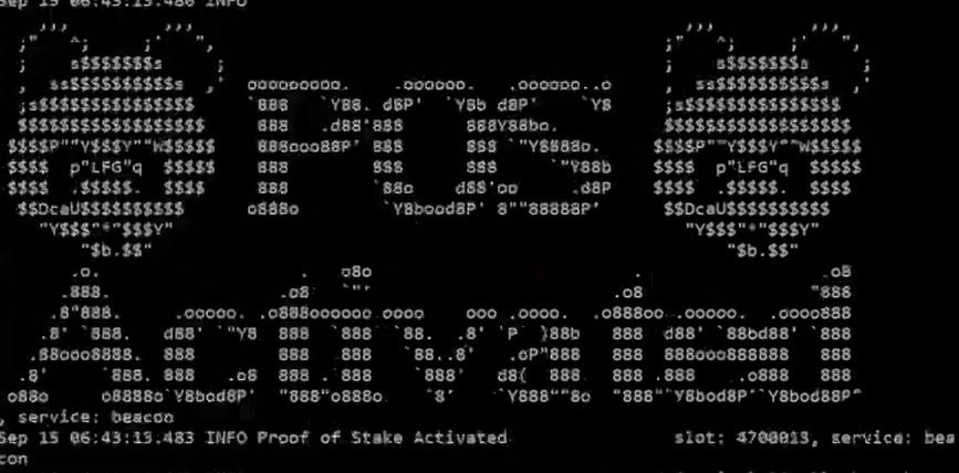
After the Merge, big stakers have a high chance of proposing multiple blocks in a row, which makes manipulation back to the initial price possible and significantly lowers the attack cost. It also makes TWAPs cheaper to move, as the attacker can maintain the manipulated price for longer.

Suppose the validator has $n>2$ consecutive blocks. In that case, the attacker can manipulate over $n-1$ blocks to reduce the initial capital required. In the final block $n$, they can exercise partial manipulation back to the initial price (or near it). As we have shown in Eq. (1), the final spot price to manipulate a $TWAP$ becomes closer to the initial price as the number of proposed blocks increases ($M$ in the equation). It's straightforward to show that the attack cost decreases enormously with this parameter. When protecting an oracle, we must be ready for the worst-case scenario, i.e. the post-PoS multi-block attack.

Suppose there is a delay of information (like Uniswap v3 $TWAP$) and no-arbitrage (PoS). In that case, some of the capital used for manipulation can be resold to the pool at the last block for higher values without altering the oracle price. Then, the remaining amount is collateral to default. Again, notice that borrowing to default is equivalent to selling at a diminished price due to $f$, with no price impact.

How would an optimal attack scheme look post-PoS for a validator with $n$ consecutive blocks?

1. Attack will use a total capital $C$ (measured in B): $C=C_{colateral}+C_{manipulation}$
2. With $C_{colateral}$, purchase $a_{colateral}$ of A at price $P_i$ (relative to B): $C_{colateral}=a_{colateral}P_i$. The attacker can do this over several blocks and liquidity markets to mitigate price impact.
3. With $C_{manipulation}$, manipulate the $TWAP$ to $TWAP_{final}$, by purchasing $a_{manipulation}$ of A in the AMM. The spot price to manipulate depends on the length of the TWAP queried by the market and how many blocks the proposer has at disposition.
4. Let $n-1$ block pass to register the new price.
5. Manipulate the price back in the AMM to $P_f'=f*TWAP_{final}$ by selling back $a_{back}$. The attacker still holds $a_{left} = a_{manipulation}-a_{back}$. Notice $a_{left}$ is equivalent to the amount out of manipulating the pool up to $P_f'$.
6. In the same block, deposit $a_{colateral}+a_{left}$ as colateral and borrow asset B with borrowing capacity $f(a_{colateral}+a_{left})TWAP_{final}$. Notice the reserves cap this amount.
7. Default bad debt and profit.

$a_{colateral}$ and $a_{manipulation}$ should be chosen to maximize the reserves. Demanipulating further would be equivalent to selling for a lower price.

$Profit = min[(a_{colateral}+a_{left})f*TWAP_{final},Reserves+SoldBack]-a_{colateral}P_i-C_{manipulation}'$

where $C_{manipulation}'$ corresponds to the cost of manipulating up to $P_f'$ and $SoldBack$ the remaining capital sold back to the pool (only greater than zero if reserves were exhausted).

An attacker could also manipulate the TWAP without getting arbitraged if they propose several non-consecutive batches of blocks where they must sacrifice the final block of each batch to close the manipulation.

You can play around with a simulation for this attack here and generate plots for different variables. The absence of arbitrage in this scenario makes everything smoother from the attacker's perspective. This attack can reach profitability quite easily, even after considering the TWAP.

The equilibrium price is a function of $a_{colateral}$. The higher this capital, the lower the target $TWAP$ (but also, the less profit). For significant enough price manipulations, $a_{left}$ is sufficient to be profitable, and $a_{colateral}$ might be unnecessary. This dependence with $a_{colateral}$ complicates the use of almost Full Range positions as a more efficient alternative to Full Range positions.

This scheme requires an additional up-front capital $a_{back}$ , which is trivially recovered by manipulating back, but it's also the heaviest capital. The up-front cost falls exponentially with the attack length (number of consecutive blocks to propose). The longer the $Lenght_{TWAP}$ the market uses relative to the attack length $Length_{attack}$, the more serious this capital becomes.

⚠️ This attack can easily reach profitability. Increasing the TWAP parameters will only require the attacker to have a more significant up-front capital (redeemable after the attack).

⚡ So, we are in danger once again… unless we use PRICE 🧠

Conclusion

This article has gone through the basic definitions of Uniswap v2 and v3. We have computed the cost of manipulation in each case. We have also discussed the $TWAP$ price and its parameters.

We then showed that previous to the PoS consensus, an attack on a lending market could be profitable only if the market used the spot price as an oracle or the liquidity was in an unhealthy shape, either by lousy deployment or absence in secondary markets.

With the recent switch to PoS, TWAP oracle manipulation has become profitable again, even for pools with healthy liquidity. Multi-block proposing allows attackers to filter away interactions with a specific pool during their proposing window. A new approach is necessary to keep using Uniswap TWAPs after the Merge, which PRICE brings to the table.

The following post will discuss the parameter selection used to design PRICE.

You can reach out to us on Twitter if you have any questions.

Price

Special thanks to Guillaume Lambert and Gaston Maffei for the review and feedback.